

This paper presents a hybrid deep-learning approach to malware detection that employs the use of a diverse set of eight unique malware datasets. Figure 1 shows a visual illustration of the process of the proposed paradigm.
Proposed BEFSONet malware detection model.
In the first step, the datasets are loaded into data frames and combined according to the target column. This allows for the separation of harmful and benign occurrences for further analysis using graphical data analysis. We take mreasures to mitigate overfitting by thoroughly analyzing the spread of the target variable, recognizing that imbalances in datasets could lead to challenges. Following that, The input data is converted into a structure that can be processed by DL using Single Hot Encode and Feature Engineering. Next, using feature scaling, the data is normalized and aligned with the typical range of independent variables. When dealing with vast volumes of data, the Zeek Analysis Tool (ZAT) data frame is useful since it contains essential aspects that are found by using the Mean of Reduction in Accuracy (MDA) and RF techniques. The DBSCAN method is used to cluster the information, and the silhouette rating metric is used to evaluate the effectiveness of various clustering strategies. The isolation tree approach is used to find any differences or abnormalities in the dataset after the clustering phase. After completing these preparation processes, DL analysis is performed on the dataset. Before classification, we divided the data into two parts: 80 percent is test data, and 20 percent is training data. The SHO optimization method is used to optimize BEFSONet parameters, which are essential for improving classification.
Dataset collection and description
IoT 23 is a significant resource that was created particularly to gather network packets flow from the IoT devices. Twenty distinct scenarios are included in this dataset, which include both instances of malware-induced IoT device compromise and benign IoT traffic43. These scenarios are methodically organized and include three legitimate network traffic samples from common IoT devices, as well as an additional twenty pcap files depicting scenarios involving compromised devices. Particularly, the pcap files are modified every 24 hours, a metric ascribed to the malware’ dynamic nature and the significant traffic created during each transmission. However, it is important to emphasize that several pcap files had to be stopped for over a day owing to their large size, resulting in variances in capture lengths.
Table 2 contains detailed information on the 20 scenarios, including ID_scenario, name of dataset, length(hours), transaction count, ID_Zeek, and information collected from the conn.log document using Zeek’s network analysis framework. The table also provides details regarding the size of the pcap files as well as probable names connected with the variants of malware used to infect each device. The IoT 23 dataset is valuable because it has the potential to assist researchers and developers working on security projects by offering a platform for improving detection models and machine-learning algorithms. With its wide range of network traffic situations, it is an invaluable tool for education, helping with the teaching and assessment of security solutions.
Stratosphere laboratories carefully craft the labels in the IoT-23 dataset through a detailed examination of malware captures, which allows them to describe connections that are linked to illegal or potentially hazardous activity. These labels are important identifiers of malicious traffic, typically revealing patterns of activity43. The term “attack” describes efforts to take advantage of weak services on hosts other than the compromised device. Flows that show attempts to take advantage of weak services, such as brute force telnet login attempts and GET request header command injection assaults, are included in this category. Conversely, connections with no questionable or dangerous behavior are indicated by the Benign designation. Control and Communication (C &C) servers are connected to devices with the C &C designation. Frequent visits to fraudulent websites, file downloaded files, or the discovery of encoded or IRC-like instructions are indicators of this activity. The Distributed Denial of Service (DDoS) label indicates that the compromised device is launching a DDoS assault, sending several data streams to a single IP address.
FileDownload refers to connections where files are downloaded to devices that have been hacked. Identifying these associations entails closely examining communications with address bytes greater than 3KB or 5KB, frequently focusing on certain dubious ports for destinations or IPs connected to C &C servers. Connections that are identified by the HeartBeat tag enable the C &C server to keep an eye on the compromised host. These connections are often identifiable and associated with response data smaller than one kilobyte (KB). Connections that meet the requirements for a Mirai botnet-a common attack vector-are designated with the Mirai label. Similar to Mirai, but with lower frequency, the Okiru label indicates connections suggestive of an Okiru botnet. The parameters for classification are comparable to those employed in the case of Mirai.
Horizontal port scans are used to get information about impending attacks on connections identified with the PartOfAHorizontal-PortScan label. Recognizing patterns where connections share a range of IP addresses, utilize the same port, and transfer almost the same amount of data is necessary to detect these connections. Connections with the Torii identification are considered to be a component of the Torii botnet, which is distinguished from Mirai by being less widespread yet adhering to similar criteria. Together, these classifications help provide a more complex picture of the risks included in the IoT-23 dataset.
Pre-processing
Prior to implementing classification algorithms, we employed several data analysis and preparation approaches. The goal column was later added when all the data were first combined into the same data frame. The subsequent sequence, which we explored into in greater detail, was followed in completing the preprocessing steps.
In preprocessing, when a binary classification method is used to determine whether an instance is malignant (1) or benign (0), it becomes crucial to understand the pattern of distribution of a target parameter in the identification of malware. A ML model’s effectiveness depends on the target variable’s distribution being balanced; a skewed distribution, in which one class predominates, might result in erroneous model predictions. For instance, a model might achieve a 95% accuracy rate by consistently predicting the majority class when 95% of the samples are benign, overshadowing potential malicious instances44.
Metrics to measure this distribution include the number of examples in each class, the average and variance of the target parameter, and the fraction of malicious samples (p). The proportion of malicious samples is calculated by \(p = \frac{n_{\text {malicious}}}{n_{\text {total}}}\), where \(n_{\text {malicious}}\) and \(n_{\text {total}}\) indicate, respectively, the quantity of malicious observations and the overall number of instances. The mean (mean) and variance (variance) are derived using the following formulas44:
$$\begin{aligned}{} & {} \text {mean} = \frac{n_{\text {malicious}} \times 1 + n_{\text {benign}} \times 0}{n_{\text {total}}} \end{aligned}$$
(1)
$$\begin{aligned}{} & {} \text {variance} = \frac{n_{\text {malicious}} \times (1 – \text {mean})^2 + n_{\text {benign}} \times (0 – \text {mean})^2}{n_{\text {total}}} \end{aligned}$$
(2)
These statistical measures provide insights into the distribution characteristics, offering valuable information for evaluating the ML model’s efficiency in identifying malware.
Feature representation through one hot encoding
Within our malware dataset, each sample is categorized into distinct malware classes. Utilizing one-hot encoding, an 8-bit vector is generated for each malware type, with each position in the vector corresponding to a potential class45. This encoding methodology ensures that each malware type is uniquely represented in a binary format. One-hot encoding, for instance, would encode malware types X, Y, and Z as [0, 1, 1], [1, 0, 1], and [1, 1, 0], respectively. Each sample in the dataset is then transformed into a one-hot encoded vector, signifying its respective malware class. This encoding facilitates the input of malware labels into machine-learning models, allowing for effective pattern recognition and interrelation analysis across various malware strains.
Standardization of features via feature scaling
In our malware dataset, samples are characterized by features related to distinct malware types. These features, however, often exhibit varying scales, posing a challenge for comparative analysis. Scaling of features becomes crucial as it standardizes a range of attributes and enable predictive algorithms to derive more pertinent information from the data set46.
Feature scaling involves standardizing feature values within a range of 0 to 1, thereby enhancing comparability and analysis across diverse features. The normalization equation is expressed as46:
$$\begin{aligned} x’ = \frac{x – x_{\text {min}}}{x_{\text {max}} – x_{\text {min}}} \end{aligned}$$
(3)
The normalized values of the feature x is denoted by \(x’\) in this equation, whilst the dataset’s lowest and highest values for that particular attribute are represented by \(x_{\text {min}}\) and \(x_{\text {max}}\). Feature scaling is a technique that enhances ML models’ ability to detect and classify malware. By ensuring that all characteristics are on a same size, this standardization helps ML algorithms operate better and produce better results when applied to the dataset.
Feature scaling
Within our malware dataset, we have samples categorized under Mirai and Kenjiro, each associated with distinct malware types. These features often exhibit varying ranges, posing a challenge when it comes to comparative analysis. Feature scaling, a process of standardizing these values, proves instrumental in allowing ML algorithms to glean more meaningful insights from the data46. Our approach involves normalizing the feature values to a standardized range of 0 to 1, thereby enhancing their usability. The procedure unfolds as follows: The range of values for every feature found across all malware samples is computed. Next, the normalization Eq. (4) is applied to each unique feature value46.
$$\begin{aligned} y’ = \frac{{y – y_{\text {min}}}}{{y_{\text {max}} – y_{\text {min}}}} \end{aligned}$$
(4)
In this case, an attribute’s starting value is indicated by \(y\), its lowest value in the dataset is indicated by \(y_{\text {min}}\), its greatest value is shown by \(y_{\text {max}}\), and its standardized value is indicated by \(y’\). Feature scaling guarantees that all characteristics are brought to the same scale, which makes accurate comparisons and analyses possible. Consequently, this leads to improved accuracy and performance when machine learning techniques are used on the dataset.
Analyze an example containing a sample linked to the virus Mirai, whereby Kenjiro = 60 and Mirai = 100. Each value in the dataset can have its own normalization equation applied to it if the lowest and highest values for the Mirai attribute are 60 and 450, and the maximum values for Kenjiro are 25 and 250, respectively.
$$\begin{aligned} \text {{Mirai}}’ = \frac{{100 – 60}}{{450 – 60}} \end{aligned}$$
(5)
This signifies that the standardized measurement of the Mirai characteristic for this instance is 0.1877. A similar calculation can be performed for the Kenjiro feature:
$$\begin{aligned} \text {{Kenjiro}}’ = \frac{{60 – 25}}{{250 – 25}} \end{aligned}$$
(6)
This produces a value of 0.328, meaning that this sample’s average Kenjiro attribute score is 0.328. The effectiveness of machine learning techniques utilized in malware recognition and identification is increased by using feature normalization in our malicious sample dataset. By ensuring that different feature properties are integrated into a uniform scale, this strategy improves the overall efficacy of machine learning strategies that are used for malware identification and classification.
Extraction of features by RF significance
Recognizing the meaning of characteristics is essential to understanding the mechanics of decision-making in machine learning models. This knowledge enables us to identify the characteristics that have a significant impact on a model’s predictions. Understanding feature relevance in detection of malware is essential for recognizing critical characteristics or indications that are necessary for precise malware categorization.
The Mean Reduction in Efficiency (MDA) technique is used by the random forest strategy, that is well known for producing effective malware models for detection47. Machine learning evaluates a feature’s significance by calculating the overall accuracy reduction caused by splitting data based on a certain attribute. We examine the MDA scores attributed to each of the critical features necessary for efficient malware identification.
The following stages are involved in using MDA to determine the relevance of features while creating a Random Forest model for malware detection:
-
Create a Random Forest model by utilizing the training set of data.
-
To obtain a range of relevance scores for features, access the trained model’s “importance_attribute” attribute.
-
To determine which features are most important, the attribute importance scores are arranged in chronological order.
By examining those scores, we are able to identify critical characteristics or indicators that are essential for effective malware identification.By leveraging this data, we can enhance the performance of our ML approaches and boost its accuracy in identifying malware. Setting these crucial malware indications as priorities greatly improves the model’s detection performance47. Moreover, our method extends to model optimization by locating and removing unnecessary or redundant components. This process of streamlining leads to a more streamlined framework for identifying and categorizing malicious instances, diminishing the intricacies of the system and enhancing its efficacy.
ZAT to dataframe to matrix
The Zeek Access program (ZAT), a program in Python intended for malware research and representation, is utilized to apply the DataFrame to Matrix technique. Using malware data, this technique converts a Data Frame into a matrix representation48. Before proceeding on, the data must be converted into a two-dimensional set of integers. This entails employing one labeling coding approaches to represent data into categories, then scaling the numerical data to create a level distribution and variance. When the information is in matrices form, data can be put into various algorithms using machine learning for classification. The mathematical transformation of a data frame into a matrix representation is depicted in Eq. (7). Each column represents an attribute, and each entry corresponds to an observation. Let \(A\) symbolize the original dataset with \(p\) instances and \(q\) attributes48.
$$\begin{aligned} B = [a_1, a_2, \ldots , a_p] \end{aligned}$$
(7)
Specifically, \(g_t\) represents the \(t\)-th attribute in \(B\), and \(B’\) represents a matrix representation of \(B\), as stated in Eq. (8), where every line indicates an instance and every column indicates an attribute48.
$$\begin{aligned} B’ = \begin{bmatrix} g_1(a_1) &{} g_2(a_1) &{} \ldots &{} g_q(a_1) \\ g_1(a_2) &{} g_2(a_2) &{} \ldots &{} g_q(a_2) \\ \vdots &{} \vdots &{} \ddots &{} \vdots \\ g_1(a_p) &{} g_2(a_p) &{} \ldots &{} g_q(a_p) \end{bmatrix} \end{aligned}$$
(8)
\(g_i(a_j)\) indicates the value that was assigned to the \(i\)-th property for the \(j\)-th occurrence. Considering the traits inherent in the features of the initial Data Frame, diverse approaches can be utilized to preprocess and transform the data prior to its conversion into matrix form.
Clustering with DBSCAN for malware analysis
Malware isntances with similar features are grouped together by applying clustering approach i.e, DBSCAN49. This approach enhances the ability to identify distinct patterns in the data, aiding in the recognition of various malware strains such as Mirai, Kenjiro, Linux Hajime, Okiru, among others.
The first step in integrating DBSCAN into identifying malware is preprocessing the malware sample’s dataset and feature engineering it. In order to simplify the space for features, the next step needs to use Principal Component Analysis (PCA). This includes identifying a collection of parallel lines that best reflect the variability in the data. Malware samples are then clustered using DBSCAN clustering based on the reduced depictions of features.
DBSCAN clustering works by grouping a dataset \(A\) including \(p\) malware instances with \(q\) features into clusters \(D_1, D_2, \ldots , D_k\). The method is described in Eq. (9)49, whereby the sum of the squared variations between each malware occurrence and its assigned centroid are lowered.
$$\begin{aligned} \text {Minimize} \sum _{i=1}^k \sum _{a=0}^k a^j \in D^i ||A^j-\mu ^i ||^2 \end{aligned}$$
(9)
In this case, \(D_i\) represents the set of samples for malware assigned to cluster node \(i\).
PCA
The PCA methods utilized to create a new data/information of \(r\) attributes by taking data from the dataset \(A\) of \(p\) samples of malware with \(q\) traits. The goal, as shown by Eq. (10), is to maximally capture the variability in the data.
$$\begin{aligned} B = AW \end{aligned}$$
(10)
The matrix denoted by \(W\) in this equation is one in which the diagonal eigenvector of the matrix of covariance of \(A\) coincide with the eigenvalues of \(k\) that are most important. Malware samples have been arranged closely to show previously unidentified categories like Kenjirro, Linux Hajimee, Okirru, and Miraii through integrating DBSCAN with PCA. This approach significantly advances vulnerability analysis, detecting malware, and cybersecurity.
Silhouette score
An important statistic for evaluating clustering efficacy is the Silhouette Score, which evaluates how effectively clusters are created as well as how accurately cluster instances are categorized. A high Silhouette Index denotes successful malware grouping, which makes it easier to discover new malware variants through classifying samples according to common characteristics. Equation (11)50 expresses the mathematical calculation of the silhouette factor for each occurrence \(J\) in \(A\).
$$\begin{aligned} \text {sc}(k) = \frac{w(k) – z(k)}{\max [z(k), w(k)]} \end{aligned}$$
(11)
In this case, the average difference to all instance in other clusters is indicated by \(w(k)\), while \(z(k)\) is the mean difference among all occurrences within the same cluster. In clustering evaluations, the silhouette coefficient offers information about the quality of the clusters generated by measuring the degree to which instances mesh inside the cluster and the degree to which clusters are effectively divided.
Proposed ensemble model: BEFSONet
The main classifier in this paper is BEFSONet, and the optimization approach is ensemble. Additionally, cutting edge ML and DL approaches have been used to validate the hybrid method. Below is a discussion of the models with a detailed description.
BERT-feed forward neural network
In the initial phase of the BERT-Feed Forward Neural Network (FFNN) ensemble for malware classification, a crucial step involves tokenization. Malware instances undergo tokenization using the BERT tokenizer, which can be represented as:
$$\begin{aligned} \text {Tokens} = \text {BERT\_Tokenizer}(\text {Malware Instances}) \end{aligned}$$
(12)
Following tokenization, the contextual embeddings \(E_{\text {BERT}}\) are obtained using BERT51. These embeddings are more than static representations; they capture the nuanced relationships and meanings of words within the sequence. BERT’s contextual embeddings provide a comprehensive representation by considering the context of each word in relation to the entire sequence:
$$\begin{aligned} E_{\text {BERT}} = \text {BERT}(\text {Tokens}) \end{aligned}$$
(13)
The BERT-FFNN ensemble leverages these contextual embeddings from BERT as the input layer for the subsequent Feed Forward Neural Network (FFNN)52. The FFNN is a key component that adds a layer of pattern-learning capabilities to the model. In the FFNN, the contextual embeddings are processed through fully connected layers, each equipped with an activation function such as ReLU:
$$\begin{aligned} Z_{\text {FFNN}} = \text {ReLU}(\text {W}_{\text {FFNN}} \cdot E_{\text {BERT}} + \text {b}_{\text {FFNN}}) \end{aligned}$$
(14)
Due to its design, the model is capable of picking up on complex patterns and characteristics seen in the specific embeddings, which helps to provide a more thorough knowledge of the malware cases. To create a cohesive ensemble, the outputs from both BERT and the FFNN are fused using a predefined ensemble strategy. This strategy, which could involve a weighted combination of the two outputs, allows for the flexible integration of the strengths of each model:
$$\begin{aligned} \text {Ensemble Output} = \alpha \cdot \text {Output}_{\text {BERT}} + (1 – \alpha ) \cdot \text {Output}_{\text {FFNN}} \end{aligned}$$
(15)
The value of the hyperparameter \(\alpha\) in this case controls the degree of importance given to the BERT outcome in the end result ensemble output.
The training phase involves fine-tuning BERT for the specific context of malware classification and optimizing the parameters of the FFNN through backpropagation. The classification loss, which is determined by analyzing the ensemble output with the base truth labels, guides the optimization process:
$$\begin{aligned} \text {Loss} = \text {Compute\_Loss}(\text {Ensemble Output}, \text {Ground Truth Labels}) \end{aligned}$$
(16)
After then, the algorithm’s efficiency is assessed using common metrics like as F1 score, accuracy, precision, and recall. Continuous model optimization may involve hyperparameter change, such as changing the weight assigned for the BERT outcome (\(\alpha\)) and testing with various ensemble configurations. The BERT-FFNN ensemble is fine-tuned to be suitable for the malware identification job through this iterative method, integrating its advantages of embedded context with pattern-learning skills for consistent results.
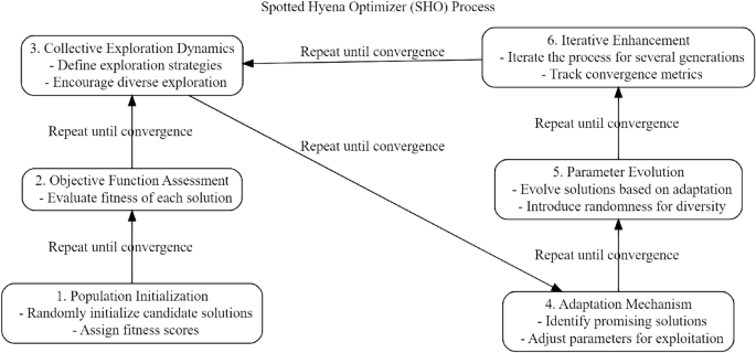
Spotted hyena optimizer (SHO)
SHO is an optimization technique derived from nature, mimics the eating patterns of hyenas with spots in their natural environment53. The main purpose of this optimization technique is to improve the performance of the model by adjusting the BERT-FFNN ensemble’s variables for malware classification. The SHO algorithm is modeled after the effective cooperation of spotted hyenas during cooperative hunting to capture prey. Similarly, SHO cooperates and adjusts when changing the parameters of the BERT-FFNN ensemble to enhance the general efficacy of the model.The primary components and methods of the SHO for modifying BERT-FFNN settings are as follows53:
-
We start with a population P representing potential solutions, where each solution \(s_i\) corresponds to a unique set of parameters for the BERT-FFNN ensemble:
$$\begin{aligned} P = {s_1, s_2,…, s_n} \end{aligned}$$
(17)
-
Objective Function Assessment: The objective function \(J(s_i)\) evaluates the performance of the BERT-FFNN ensemble with the specific set of parameters \(s_i\)53:
$$\begin{aligned} J(s_i) = \text {Evaluate BERT-FFNN performance with parameters } s_i \end{aligned}$$
(18)
-
Collective Exploration Dynamics: Solutions dynamically share insights, updating their knowledge by incorporating information from other solutions. The collaborative exploration equation becomes53:
$$\begin{aligned} s_i^t = s_i^{t-1} + \alpha \cdot (s_j^{t-1} – s_k^{t-1}) \end{aligned}$$
(19)
where \(s_i^t\) represents the updated solution, \(\alpha\) is the learning rate, and \(s_j^{t-1}\) and \(s_k^{t-1}\) are solutions from the previous iteration.
-
Adaptation Mechanism: The search space adapts based on collective knowledge, adjusting solutions in the direction of the objective function gradient53:
$$\begin{aligned} s_i^{t+1} = s_i^t + \beta \cdot \nabla J(s_i^t) \end{aligned}$$
(20)
Here, \(\beta\) controls the step size, and \(\nabla J(s_i^t)\) is the gradient of the objective function.
-
Parameter Evolution: BERT-FFNN ensemble parameters evolve by assimilating shared information, ensuring the model adapts to the collaborative insights and Adjust parameters of BERT-FFNN using knowledge from P.
-
Iterative Enhancement: The iterative refinement persists until an optimal parameter configuration is achieved, ensuring the BERT-FFNN ensemble performs optimally:
$$\begin{aligned} \text {Repeat until convergence: } P = \text {SHO}(P) \end{aligned}$$
(21)
This adaptive and collaborative optimization process enhances the exploration of the parameter space, facilitating the BERT-FFNN ensemble’s ability to effectively capture intricate features in malware instances. The process of SHO is shown in Fig. 2.
Interpretability and explainability
For the BEFSONet architecture to be practically useful in actual IoT security scenarios, it is imperative that it be comprehensible and easy to understand. In this instance, this study explores the ease with which domain experts may comprehend and interpret the model’s judgements, placing a focus on transparency and reliability.
Model decision interpretability
To deliver reliable IoT security solutions, BEFSONet uses a BERT-based Feed Forward Neural Network Framework (BEFN) optimised with the Spotted Hyena Optimizer. The model’s architecture is made to recognise complex patterns in IoT security data, which makes it quite good at categorising different kinds of malware. The following essential elements make BEFSONet’s decisions easier to interpret:
-
1.
Feature Importance Analysis: The model employs feature crafting techniques, such as thorough category encoding and feature normalisation. By using RF and MDA studies, BEFSONet highlights and finds the most important features influencing its conclusions.
-
2.
Ensemble Methodology: To further improve interpretability, BEFSONetO, an avant-garde DL ensemble, is used. The ensemble technique facilitates understanding of the rationale behind the final categorization by providing a collective choice by aggregating the outputs of numerous algorithms.
Explainability mechanisms
BEFSONet possesses strategies to explain its forecasts in order to promote trust and ease model adoption:
-
Attention Mechanisms: By utilizing BERT’s attention mechanisms, BEFSONet brings focus to particular input data points that are crucial to the model’s conclusion. This explanation based on attention provides information on which features are considered most important for a certain prediction.
-
SHAP (SHapley Additive exPlanations): To measure each feature’s effect on the model’s output, BEFSONet uses SHAP values. This methodology guarantees an equitable distribution of significance among distinct attributes, contributing to the decision-making process’s overall comprehensibility.
Fine-tuning BEFSONet parameters with SHO
Achieving optimal performance in the BERT-Feed Forward Neural Network (BEFSONet) for malware classification demands meticulous parameter tuning. The Spotted Hyena Optimizer (SHO) emerges as a potent metaheuristic algorithm employed to automatically fine-tune the diverse parameters governing the BEFSONet. This section delves into the intricacies of integrating SHO into the parameter optimization process. The tuning parameter flow is shown in Fig. 3.
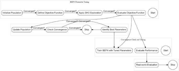
Internal process of tuning with SHO.
Navigating the Parameter Landscape The parameters steering the BEFSONet’s behavior encompass learning rates, batch sizes, dropout rates, and other hyperparameters. Aptly configuring these parameters holds the key to expedited convergence, swifter training cycles, and an overall improvement in model efficacy.
Synergy of SHO and BEFSONet: Harmonizing SHO with BEFSONet parameter tuning unfolds through a systematic sequence:
-
1.
Initial Parameters: Set the initial population of candidate solutions, representing distinct parameter configurations for the BEFSONet.
-
2.
Objective Function Crafting: Using specified evaluation criteria, such as precision, recall, preciseness, or F1 score, create an objective function that measures BEFSONet’s performance.
-
3.
SHO Optimization Loop: Immerse the SHO algorithm in an iterative exploration-exploitation dance within the parameter space. Dynamically adjusting parameters seeks optimal values that refine the objective function.
-
4.
Performance Evaluation: Measure BEFSONet’s performance with the tuned parameters on a validation set. If convergence criteria are met, proceed; else, loop back to the SHO optimization stage.
-
5.
Training the Tuned Model: Train the BEFSONet with the best-tuned parameters on the complete training dataset.
-
6.
Real-world Evaluation: Assess the final BEFSONet model’s generalization and performance on an independent test set, mimicking real-world scenarios.
SHO’s contribution in Parameter Tuning: The advantages SHO brings to the table for BEFSONet parameter tuning are significant:
-
Global Exploration Prowess: SHO’s exploration strategy systematically canvasses the parameter space, sidestepping local optima traps.
-
Adaptive Precision: SHO dynamically adapts its exploration-exploitation balance, focusing on promising parameter areas as the optimization journey unfolds.
-
Swift Convergence Dynamics: SHO’s iterative nature ensures a streamlined convergence towards optimal or near-optimal BEFSONet parameter configurations.
-
Automation Efficiency: SHO’s automation prowess minimizes manual intervention, expediting the parameter optimization journey.
Incorporating SHO into the BEFSONet parameter tuning process stands as an automated and efficient strategy, uncovering optimal hyperparameter tuning that significantly enhance the malware classification model’s effectiveness. The pseudocode of tuning process is shown in Algorithm 1.
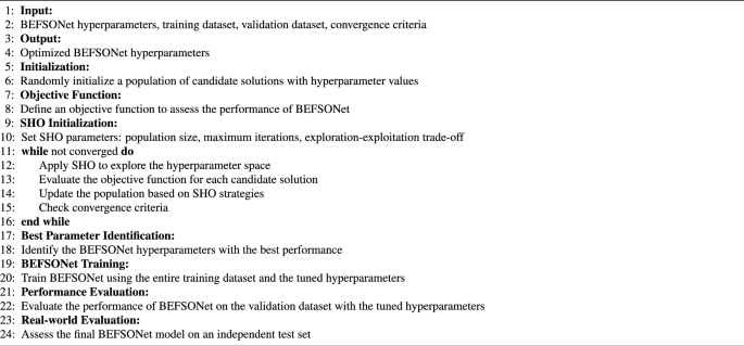
BEFSONet parameter tuning with SHO.

Tyler Fields is your internet guru, delving into the latest trends, developments, and issues shaping the online world. With a focus on internet culture, cybersecurity, and emerging technologies, Tyler keeps readers informed about the dynamic landscape of the internet and its impact on our digital lives.